Multi-head Latent Attention
This is a note about DeepSeek-V2 Multi-Head Latent Attention.
Introduction
Large Language Models (LLMs) operate on a simple principle: Autoregressive Decoding. This means that the model generates text one token at a time, using the entire history of the conversation to predict the next word. However, this comes with a significant computational cost. To generate N-th token, the model needs the information of all previous N-1 tokens. Re-computing the entire attention states (Key and Value) at every single step would be prohibitively slow.
To address this issue, we usually use KV Cache to store the Key(K) and Value(V) vectors of all previous tokens in VRAM. At each decoding step, we only need to compute the K and V vectors for the current token, and append them into the KV Cache.
While caching K and V avoids re-computing, it introduces a memory bottleneck that scales linearly with sequence length:
In practice, modern LLM inference is often memory-bandwidth bound rather than compute-bound, especially during long-context decoding stage.
While attention computation itself is highly optimized, repeatedly reading and writing large KV cache from GPU memory becomes the bottleneck. This observation motivates a series of techniques to reduce the memory footprint of the KV cache, such as MQA, GQA and MLA.
Existing KV Cache Reduction Techniques
Multi-Head Attention (MHA)
In standard multi-head attention, each attention head maintains its own key and value projections.
For a sequence of length (L) and a model with (N) layers and (H) attention heads, the KV cache stores a distinct key-value pair for every token, layer, and head.
While this design provides strong representational capacity, it leads to a large memory footprint during autoregressive decoding.
As the sequence length grows, reading and writing the KV cache becomes a dominant memory-bandwidth bottleneck.
Multi-Query Attention (MQA)
Multi-Query Attention reduces the KV cache size by sharing a single set of keys and values across all query heads.
Each attention head still computes its own query, but all heads utilize the same key-value pairs.
By removing the dependency on the number of attention heads, MQA significantly reduces the memory footprint of the KV cache.
However, this aggressive sharing limits the diversity of attention patterns across heads, which may degrade model quality in some settings.
Grouped Query Attention (GQA)
Grouped-Query Attention is similar to MQA, but it generalizes MQA by allowing multiple groups of query heads, where each group shares a set of keys and values.
where $H_{kv}$ is the number of key-value heads, and $H_q$ is the number of query heads.
Compared to MHA, GQA reduces the KV cache size by a constant factor of $\frac{H_{kv}}{H_q}$, while preserving more expressive power than MQA. We can see that GQA is a generalization of MQA. As a result, GQA has been widely adopted in large-scale models to balance memory efficiency and model quality.
Both MQA and GQA reduce the KV cache size by decreasing the number of heads stored. MLA, however, takes a completely different approach: instead of cutting down the number of heads, it changes the representation of the cache itself. The question shifts from how many heads to cache to what to cache.
Multi-Head Latent Attention (MLA)
Low-Rank Key-Value Joint Compression
The core innovation of MLA lies in its compression strategy. Unlike standard MHA where each head has a distinct projection matrix for Keys and Values, MLA projects the input hidden state into a joint compressed latent vector.
Let $h_t$ be the input hidden state at time $t$. MLA performs a down-projection to obtain the compressed latent vector $c_{\text{KV}}$:
Here, $\mathbf{c}_t^{KV} \in \mathbb{R}^{d_c}$ is the compressed latent vector, and $d_c$ is the compression dimension. Crucially, $d_c$ is significantly smaller than the total dimension of all heads in standard MHA ($d_c \ll d_h n_h$).
To generate the Keys and Values used for attention computation, we mathematically “up-project” this latent vector:
where $W^{UK} \in \mathbb{R}^{d_h n_h \times d_c}$ and $W^{UV} \in \mathbb{R}^{d_h n_h \times d_c}$ are up-projection matrices.
Moreover, in order to reduce the activation memory during training, MLA also performs low-rank compression for the queries, even if it cannot reduce the KV cache:
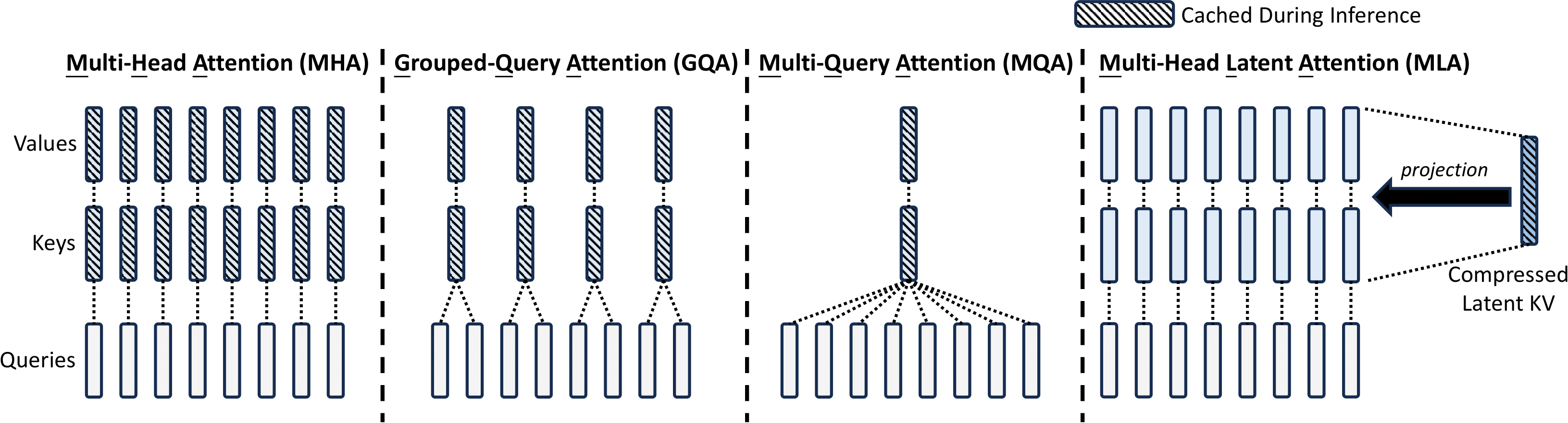
To demonstrate the difference between MHA, MQA, GQA and MLA, you can refer to the figure below:
Matrix Absorption
In addition, during inference, we can apply Matrix Absorption to reduce computation overhead.
Instead of performing the up-projections to generate the full $\mathbf{q}_{t,i}^C$ and $\mathbf{k}_{j,i}^C$ vectors, we can mathematically merge the two projection steps. Let $W^{UQ}_i$ and $W^{UK}_i$ be the up-projection sub-matrices for the $i$-th head. The attention score can be derived as the interaction between the Latent Query and Latent Key:
Here, $W_{QK,i}^{Absorbed} \in \mathbb{R}^{d_c \times d_c}$ is the pre-computed absorbed matrix for the $i$-th head.
Similarly, the Value Projection can also be optimized.
Here, we explicitly define the attention weight $\alpha_{t,j,i}$ as the Softmax of the scaled scores for the $i$-th head:
In DeepSeek-V2, the scaling factor is $\sqrt{d_h + d_h^R}$ to account for both content and RoPE dimensions (see section 3.3).
In MLA, since $\mathbf{v}_{j, i}^C$ is generated from the latent vector $\mathbf{c}_j^{KV}$, we can rewrite the output calculation:
Finally, this head’s output is projected by the output matrix $W^O$. By associativity of matrix multiplication, we can merge $W^{UV}_i$ into $W^O_i$:
Here, $\mathbf{u}_{t,i}$ denotes the output-projected representation of the i-th attention head.
The final output $\mathbf{u}_t$ is obtained by concatenating all $\mathbf{u}_{t,i}$.
Note that matrix absorption is applied only during inference. During training, we need to explicitly reconstruct the values for backpropagation.
Decoupled Rotary Position Embedding
While the low-rank compression strategy successfully reduces the KV cache size, it introduces a critical conflict with Rotary Position Embedding (RoPE).
The Conflict: RoPE vs. Matrix Absorption
As mentioned in the DeepSeek-V2 paper, standard RoPE is position-sensitive and applies a rotation matrix to the Query and Key vectors. If we apply RoPE directly to the up-projected Keys $\mathbf{k}_j^C$, the rotation matrix $\mathcal{R}_j$ (which relates to the current token position) would be inserted between the query vector and the up-projection matrix $W^{UK}$:
Because matrix multiplication is not commutative, we cannot simply move the position-dependent rotation matrix $\mathcal{R}_j$ past the fixed parameters matrix $W^{UK}$ to merge it with $\mathbf{q}$. This implies that $W^{UK}$ cannot be absorbed into $W^Q$(more precise, $W^{UQ}$) during inference. If we were to persist with this approach, we would be forced to recompute the high-dimensional keys for all prefix tokens at every decoding step to apply the correct positional rotation, which would significantly hinder inference efficiency.
The Solution: Decoupled RoPE Strategy
To resolve this, DeepSeek-V2 employs a Decoupled RoPE strategy. The core idea is to separate the query and key vectors into two parts: a Content Part for semantic features and a RoPE Part for positional information. The generation of these vectors is defined as follows:
Decoupled Queries (Multi-Head): For the queries, we generate a separate RoPE vector $\mathbf{q}_{t,i}^R$ for each attention head $i$. This maintains the multi-head diversity for positional attention.
\[ \left[ \mathbf{q}_{t,1}^R;\, \mathbf{q}_{t,2}^R;\, \dots;\, \mathbf{q}_{t,n_h}^R \right] = \mathbf{q}_t^R = \mathrm{RoPE}\!\left(W^{QR}\mathbf{c}_t^Q\right) \]Decoupled Keys (Shared-Head): For the keys, we generate a single RoPE vector $\mathbf{k}_t^R$ that is shared across all attention heads.
MLA minimizes the additional memory required to store positional information by sharing the RoPE key $\mathbf{k}_t^R$ across all heads (instead of having $n_h$ distinct RoPE keys).
Caching during inference
In MLA, we do not cache the full per-head keys/values. Instead, for each past position $j$ we cache:
- the latent KV vector $\mathbf{c}_j^{KV} \in \mathbb{R}^{d_c}$, and
- the shared RoPE key $\mathbf{k}_j^R \in \mathbb{R}^{d_h^R}$.
Final Attention Calculation
During the attention phase, the queries and keys are concatenations of their respective content and RoPE parts.
For the query at position $t$ and head $i$:
For the key at position $j$ (where $j \le t$):
The scaled attention score between query $t$ and key $j$ for head $i$ is computed as:
By expanding the dot product, we can see why MLA is efficient:
- Content Term $(\mathbf{q}_{t,i}^C)^\top \mathbf{k}_{j,i}^C$: Can be computed using Matrix Absorption (using latent vectors), avoiding explicit key reconstruction.
- RoPE Term $(\mathbf{q}_{t,i}^R)^\top \mathbf{k}_{j}^R$: Computed explicitly using the small, cached RoPE keys.
The normalized attention weights are obtained via softmax over all past positions $j$:
Finally, the attention output for head $i$ is computed using the values (which are also reconstructed from latent vectors):
The outputs from all heads are concatenated and projected to form the final output:
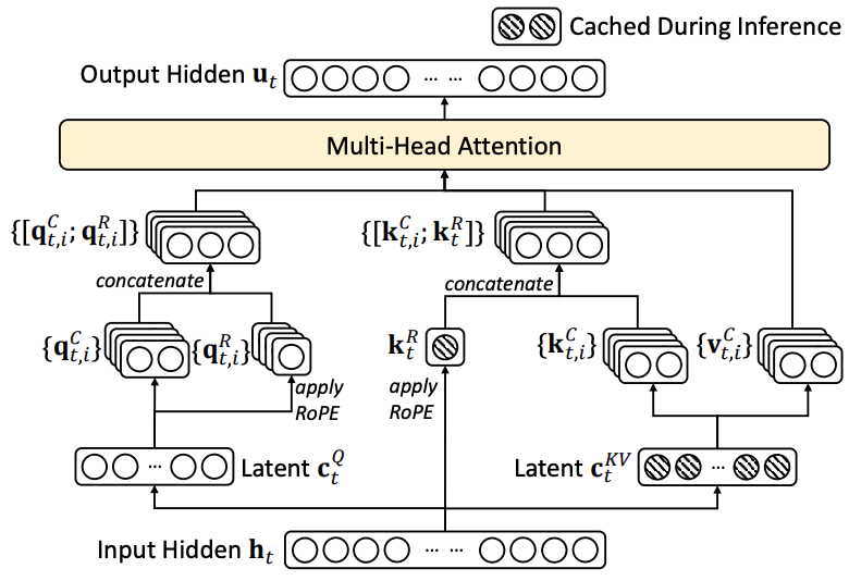
The illustration below shows the MLA flow:
Comparison of Key-Value Cache
The table below compares the KV cache size per token across different attention mechanisms:
| Attention Mechanism | KV Cache per Token (# Elements) | Capability |
|---|---|---|
| MHA | $2 \times n_h \times d_h \times l$ | Strong |
| GQA | $2 \times n_g \times d_h \times l$ | Moderate |
| MQA | $2 \times 1 \times d_h \times l$ | Weak |
| MLA | $(d_c + d_h^R) \times l \approx \frac{9}{2} \times d_h \times l$ | Stronger |
Here, $n_h$ denotes the number of attention heads, $d_h$ denotes the dimension per attention head, $l$ denotes the number of layers, $n_g$ denotes the number of groups in GQA, and $d_c$ and $d_h^R$ denote the KV compression dimension and the per-head dimension of the decoupled queries and key in MLA, respectively. The amount of KV cache is measured by the number of elements, regardless of the storage precision. For DeepSeek-V2, $d_c$ is set to $4d_h$ and $d_h^R$ is set to $\frac{d_h}{2}$. So, its KV cache is equal to GQA with only 2.25 groups, but its performance is stronger than MHA.
Reference
Multi-head Latent Attention