Roofline Model for Performance Analysis

A note about Roofline Model.

Definition

1. FLOPs : Number of Floating Point Operations. A Multiply-Add operation(MAC) is counted as 2 FLOPs.

2. FLOPS : Floating Point Operations Per Second.

   $$ \begin{aligned} \text{FLOPS} &= \frac{\text{FLOPs}}{\text{Second}} \\ \end{aligned} $$

3. OPs : Number of Operations. (Not necessarily Floating Point Operations)

4. OPS : Number of Operations Per Second.
   $$ \begin{aligned} \text{OPS} &= \frac{\text{OPs}}{\text{Second}} \\ \end{aligned} $$
5. Memory Bandwidth : The rate at which data can be read from or written to memory (Bytes per second).
6. Arithmetic Intensity : The ratio of Total OPs performed to the Total Bytes moved.
   $$ \begin{aligned} \text{I} &= \frac{C \text{(Computations, OPs)}}{M \text{(Memory Access, Bytes)}} \\ \end{aligned} $$

Process Of DNN Inference on Hardware

Step 1 (Memory Access): Moving Input/Weghts from memory to CPU/GPU.
Step 2 (Compute): Perform the operations(e.g. Linear, Convolution…).
Step 3 (Memory Access): Writing the computed activation back to memory.
The process can be visualized as below:

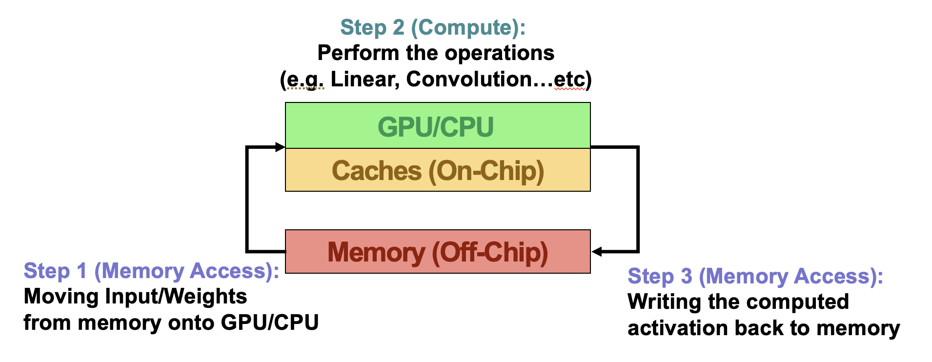
Therefore, evaluating performance requires simultaneous consideration of memory bandwidth and processing unit capabilities. If a layer involes extensive computation but minimal memory access, it is termed a computation bottleneck. Conversely, if a layer requires frequent memory access but minimal computation, it is termed a memory bottleneck. We can clearly distinguish between these two scenarios according to the Roofline Model.

Roofline Model

Plot the Roofline Model

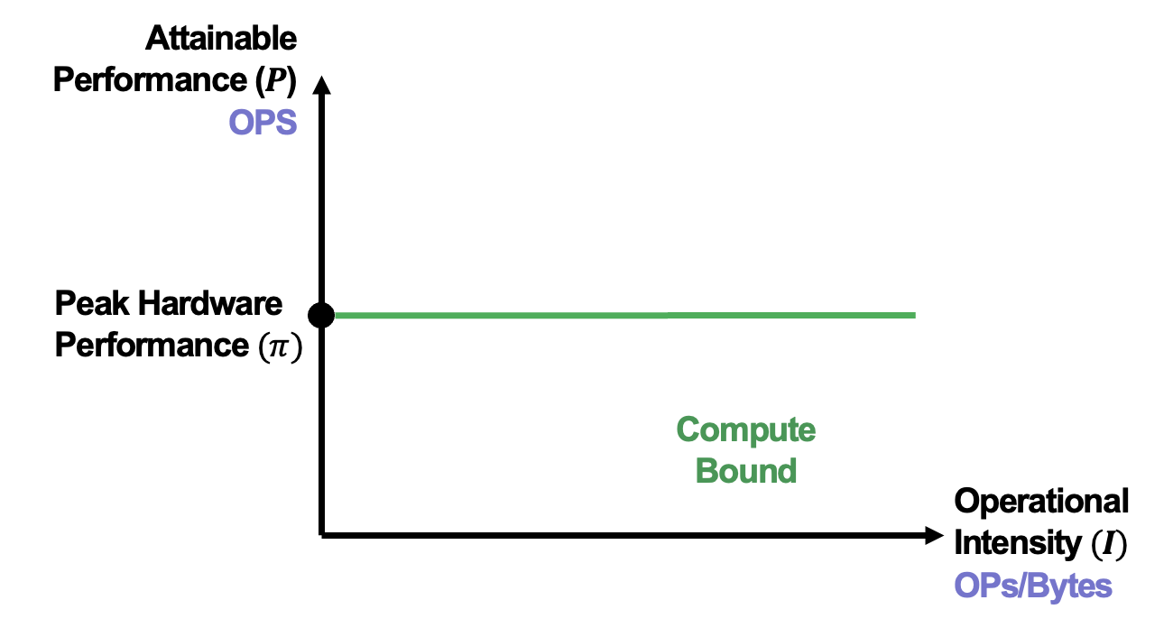
Firstly, we need to determine the Peak Computational Performance (operations per second, OPS) $\pi$ and Peak Memory Bandwidth(bytes per second) $\beta$ specific to the target hardware device. Create a graph with performance (OPS) on the y-axis and arithmetic intensity (OPs/byte) on the x-axis:

• Draw a horizontal line equal to the peak computational performance, representing the maximum achievable performance by hardware.
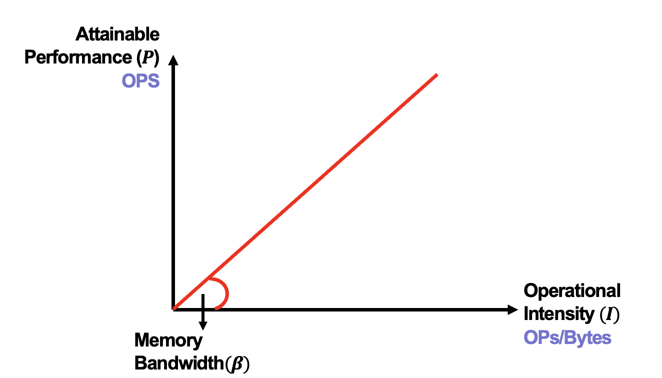
• Draw a diagonal line from the original point with a slope equal to the peak memory bandwidth, representing the maximum memory bandwidth avaible on the system.

After plotting these two lines, we can get Roofline Model as below: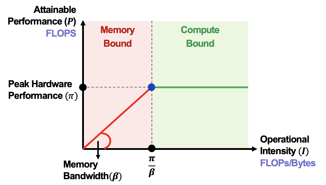

Analyze Performance for Layers

For each layer in LLMs, we can calculate its arithmetic intensity(OPs/byte) by dividing the required operations(OPs) by the amount of data transferred(bytes). According to the Roofline Model just plotted, the theoretical maximum performance for each layer is determined by the position on the graph corresponding to the arithmetic intensity of the layer. It allows us to ascertain whether this layer is compute-bound or memory-bound:

• If the layer’s arithmetic intensity is below the turning point, it means that the computational workload per memory access is low. Even saturating the memory bandwidth, it does not utilize the full computational capability of the hardware. In this case, the layer is constrained by memory access, and it is termed memory-bound. If the layer is memory-bound, we can optimize the performance by quantization, kernel fusion or increasing the batch size(decrease the number of memory access).
• Conversely, if the layer’s arithmetic intensity is above the turning point, it means that the computational workload per memory access is high. It implies that the layer requires only a small amount of memory access to consume a significant amount of computational capability, and it is termed compute-bound.

Estimated Execution Time

The execution time is the number of operations divided by performance

$$ \begin{aligned} \text{T} &= \frac{C}{P} = \frac{C}{\min(\pi, \beta \cdot I)} \\ \end{aligned} $$

Memory Bound:

$$ \begin{aligned} \text{T} &= \frac{C}{\beta \cdot I} = \frac{C}{\beta \cdot \frac{C}{M}} = \frac{M}{\beta}\\ \end{aligned} $$

Compute Bound:

$$ \begin{aligned} \text{T} &= \frac{C}{\pi} \\ \end{aligned} $$

Example Usage of Roofline Model

Here, I provide an example of using the Roofline Model to analyze the performance of a specific layer in a neural network. Suppose we have some operations with #FLOPs and #Memory Access as below:

Operation	#FLOPs (M)	#Memory Access (MB)
op1	57.8M	25MB
op2	51.4M	2.3MB
op3	925M	25MB
op4	236M	3.7MB
op5	172M	1.3MB
op6	231M	1.3MB

Reduce #Memory Access when it’s Memory Bound (op1 vs op2)

• Reducing #FLOPs results no speed up. (refer op1 and op3)
• Higher computational capability(higher $\pi$) does not improve performance.

Operation	#FLOPs (M)	#Memory Access (MB)	Operational Intensity	Attainable Performance (GFLOPS)	Theoretical Inference Time
op1	57.8M	24.5MB	2.4	226.5	255
op2	51.4M	2.3MB	22.5	2156.7	23.8
op3	925M	24.5MB	37.7	3622.6	255

Reduce #FLOPs when it’s Compute Bound (op5 vs op6)

• Reducing #Memory Access results no speed up. (refer op4 and op6)

Operation	#FLOPs (M)	#Memory Access (MB)	Operational Intensity	Attainable Performance (GFLOPS)	Theoretical Inference Time
op4	236M	3.7MB	64	4608	51.2
op5	172M	1.3MB	132	4608	37.3
op6	231M	1.3MB	174	4608	50.3

From these two scenarios, we can observe that smaller memory access or smaller FLOPs will not necessarily lead to better performance.

Conclusion

During the user’s interative with LLMs, the prefill stage excutes only once, while the decode stage is repeatedly performed to progressively generate the output. Moreover, when calculating the arithmetic intensity of each layer in LLMs, we will observe that the Prefill stage is almost entirely compute-bound, while the Decode stage is memory-bound. Therefore, optimizing for the memory bound characteristics of the decode stage becomes crucial for enhancing the inference performance of LLMs.

Reference

1. LLM Inference Unveiled: Survey and Roofline Model Insights
2. Course slides of Edge AI, NYCU.